ElasticSearch is great for indexing and searching text, but it also has a lot of functionality related to searching points and regions on the world map. In this article, we’ll learn how to index polygons corresponding to territories in the world, and find whether a point is in any indexed polygon.
Building Polygons with Geocoordinates
Back in school, we (hopefully) learned that a point in 2D space can be represented as an (x, y) pair of coordinates. A point in the world can similarly be identified by a (latitude, longitude) pair of geocoordinates. We can obtain geocoordinates for a location by clicking on the map in Google Maps or similar tools.
The analogy is not perfect though; geocoordinates are not linear, which is a result of the curvature of the Earth. This is not really important for us; the point is that we can represent any given point on the Earth’s surface by means of latitude and longitude.
Once we can identify points, it’s natural to extend the concept to 2D geometry. By taking several points, we can create polygons that mark the boundaries of a given territory, such as a country or state. Jeremy Hawes’ Google Maps Polygon Coordinates Tool is great for building such polygons.
Using this tool, we can very easily construct a rough polygon representing the state of Wyoming in the US. Wyoming is great to use as a simple example because it’s roughly rectangular, so we only need four points for a workable approximation.
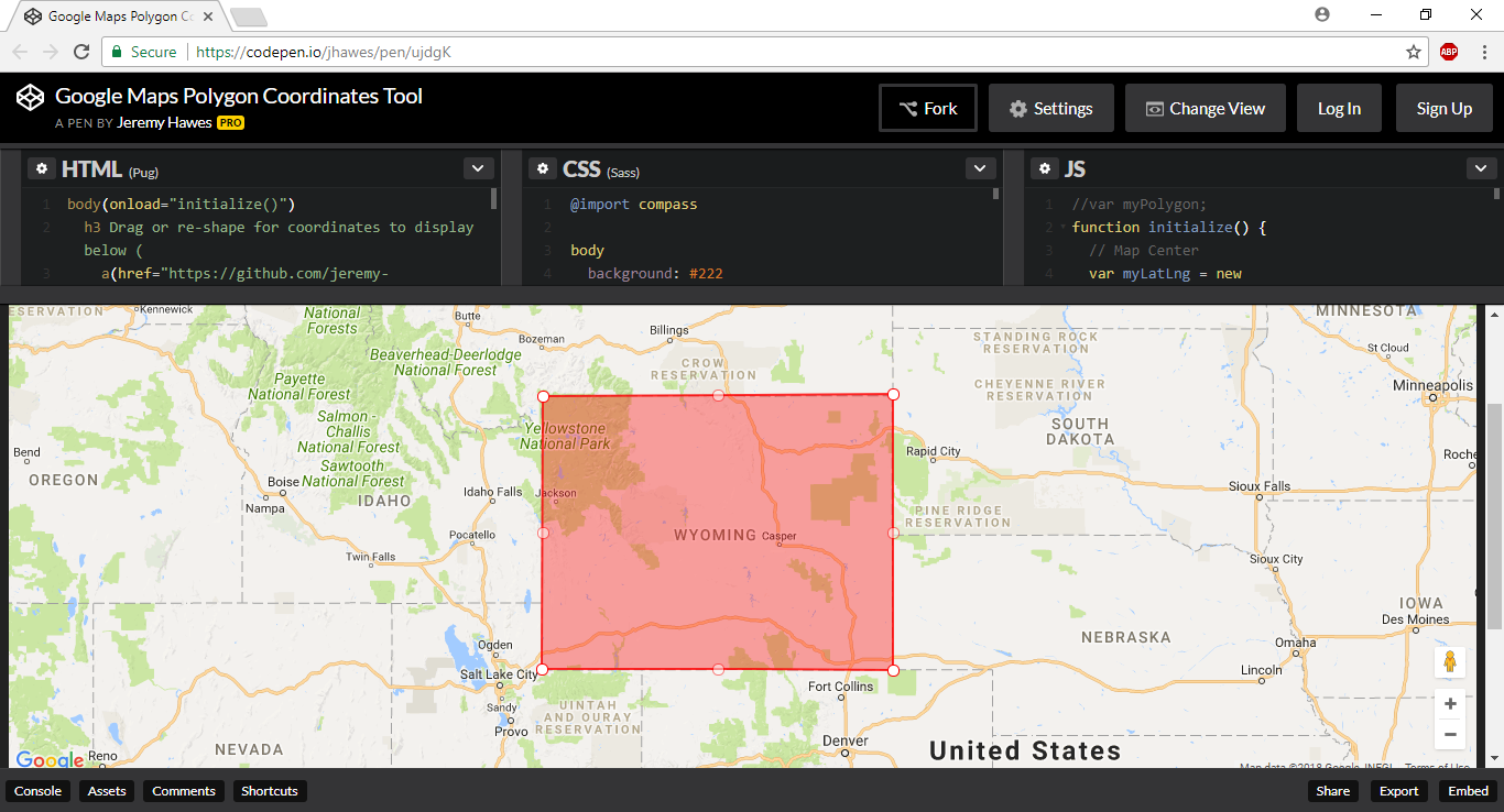
Below the map in this polygon tool, you’ll get the coordinates of the points along with some extra JavaScript (which you could later paste directly into the code editor). In this case, we’ve got the following coordinates in (latitude, longitude) format:
45.01967,-104.04405
44.99904,-111.03084
41.011,-111.04131
41.00193,-104.03375
Once we have the points that make up the polygon, we can feed them into Elasticsearch.
Indexing Geopolygons in Elasticsearch
Before we can index anything, we need to create a mapping that defines the structure of an index, including any fields and their data types. The Mapping Geo Shapes page in the Elasticsearch documentation provides a starting point. However, the documentation is crap, and if you follow the example in the docs closely, you’ll get an error:

After a quick search, this Stack Overflow answer reveals the cause of the problem: Elasticsearch no longer likes the string data type, and expects you to use text instead. This wouldn’t have been a problem if they bothered to update their documentation once in a while. Anyhow, our mapping request for this example will be as follows:
PUT /regions
{
  "mappings": {
    "region": {
      "properties": {
        "name": {
          "type": "text"
        },
        "location": {
          "type": "geo_shape"
        }
      }
    }
  }
}
This essentially means that each region item in the regions index will have a name and a location, the latter being the polygon itself. While we will be focusing exclusively on polygons in this article, it is worth noting that the geo_shape data type supports a lot of other geometric constructs – refer to the Geo-Shape documentation for more information.

Once our mapping is in place, we can proceed to index our polygons. The Indexing Geo Shapes documentation page shows how to do this. There’s a catch though: Elasticsearch expects to receive coordinates in (longitude, latitude) format, which is is the reverse of what we’ve been using so far. We can use a simple regular expression (e.g. in Notepad++) to swap our coordinates:
(\-?\d+\.?\d*),(\-?\d+\.?\d*)
\2,\1
The first line shows the regular expression that is used to match coordinates, and the second like shows what it should be replaced by, i.e. swapped coordinates.
Let’s use the following query to try to index our Wyoming polygon:
PUT /regions/region/wyoming
{
    "name" : "Wyoming",
    "location" : {
        "type" : "polygon",
        "coordinates" : [[
        [ -104.04405,45.01967 ],
        [ -111.03084,44.99904 ],
        [ -111.04131,41.011   ],
        [ -104.03375,41.00193 ]
        ]]
    }
}
This actually fails with an error:

This is because Elasticsearch expects the polygon to be closed, i.e. it must return to the starting point. Another thing to watch out for is any polygons that have self-intersections, which Elasticsearch doesn’t allow either.
We can fix our error by simply repeating the first coordinate at the end:
PUT /regions/region/wyoming
{
    "name" : "Wyoming",
    "location" : {
        "type" : "polygon",
        "coordinates" : [[
        [ -104.04405,45.01967 ],
        [ -111.03084,44.99904 ],
        [ -111.04131,41.011   ],
        [ -104.03375,41.00193 ],
        [ -104.04405,45.01967 ]
        ]]
    }
}
It should work now:

Great! Our Wyoming polygon is now in Elasticsearch.
Querying Geopolygons in Elasticsearch
We can again turn to the Elasticsearch documentation for examples of how to query our geopolygon. We can do this by taking a circle with a given radius and seeing whether it intersects the polygon, as shown in Querying Geo Shapes. Don’t confuse this with the Geo Polygon Query documentation, which is actually the opposite of our situation (i.e. having a point in Elasticsearch, and providing the polygon to test against at query time).
To test this, we’ll pick a point somewhere in Wyoming. I used Google Maps to pick a point within Yellowstone National Park, which for all we know might just be where Yogi Bear lives:
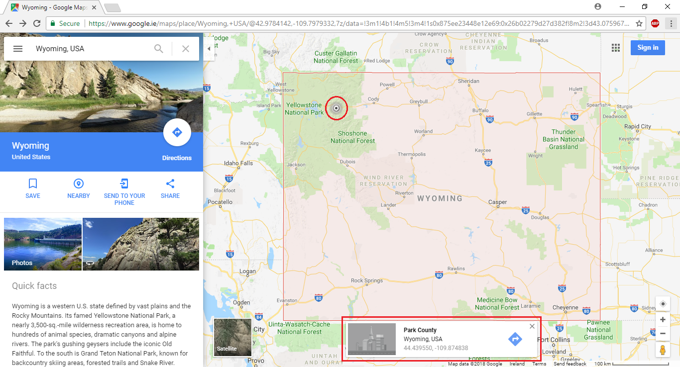
Having obtained the coordinates, we can hit Elasticsearch with a query:
GET /regions/region/_search
{
  "query": {
    "geo_shape": {
      "location": {
        "shape": {
          "type":   "circle",
          "radius": "25m",
          "coordinates": [
            -109.874838, 44.439550
          ]
        }
      }
    }
  }
}
And you’ll see that Wyoming is actually returned in the results:
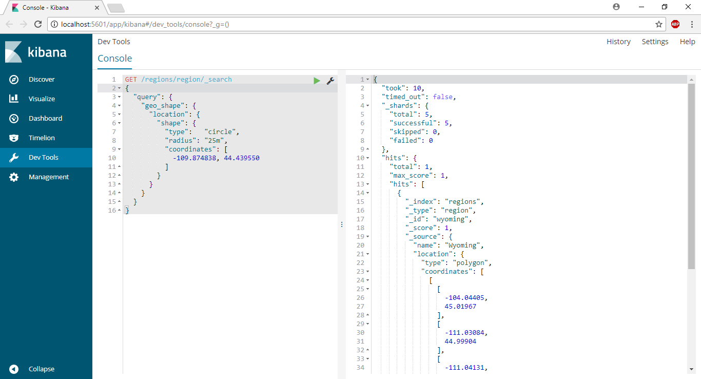
You’ll also notice that Elasticsearch gave us back all the coordinate data which we don’t really care about in this case. This can be pretty inefficient if you’re using very large and detailed polygons. We can filter that out by specifying the _source property:
GET /regions/region/_search
{
  "_source": "name",
  "query": {
    "geo_shape": {
      "location": {
        "shape": {
          "type":   "circle",
          "radius": "25m",
          "coordinates": [
            -109.874838, 44.439550
          ]
        }
      }
    }
  }
}
The results are now nice and clean:

Next, we’ll take a point in Texas and see that we don’t get results for that:

Geopolygons with Holes
Some territories aren’t simple polygons; they contain other territories inside them, and so the polygon has a hole. Examples include:
- Rome (Vatican City is a hole within it)
- New South Wales (Australian Capital Territory is a hole within it)
- South Africa (Lesotho is a hole within it)
The Indexing Geo Shapes documentation page (which we’ve referred to earlier) explains how to account for holes in polygons you index. Let’s see how this works using a practical example.

The above image shows what New South Wales, Australia looks like in Google Maps. Notice the Australian Capital Territory state inside it. Using Jeremy Hawes’ aforementioned polygon tool, we can draw a very rough polygon for New South Wales:

This gives us the following coordinates (lat, lon) for New South Wales:
-28.92704,141.04445
-33.97411,141.00841
-37.51381,149.94544
-34.98252,150.7789
-32.70393,152.18365
-28.24141,153.49901
-28.98426,148.87874
We will also need a polygon for Australian Capital Territory. Again, this will be a really rough approximation just for the sake of example:

Our coordinates for Australian Capital Territory are:
-35.91185,149.05898
-35.36119,149.14473
-35.31932,149.40076
-35.11429,149.09984
-35.3126,148.80286
-35.71989,148.81557
Next, we’ll index Australian Capital Territory. This is nothing new, but remember that we must take care to swap the coordinates so that become (lon, lat), and close the polygon by repeating the first coordinate pair at the end.
PUT /regions/region/act
{
    "name" : "Australian Capital Territory",
    "location" : {
        "type" : "polygon",
        "coordinates" : [[
            [ 149.05898,-35.91185 ],
            [ 149.14473,-35.36119 ],
            [ 149.40076,-35.31932 ],
            [ 149.09984,-35.11429 ],
            [ 148.80286,-35.3126  ],
            [ 148.81557,-35.71989 ],
            [ 149.05898,-35.91185 ]
        ]]
    }
}
For New South Wales, we do something special: we give it two polygons.
PUT /regions/region/nsw
{
    "name" : "New South Wales",
    "location" : {
        "type" : "polygon",
        "coordinates" : [
            [
                [ 141.04445,-28.92704 ],
                [ 141.00841,-33.97411 ],
                [ 149.94544,-37.51381 ],
                [ 150.7789, -34.98252 ],
                [ 152.18365,-32.70393 ],
                [ 153.49901,-28.24141 ],
                [ 148.87874,-28.98426 ],
                [ 141.04445,-28.92704 ]
            ],
            [
                [ 149.05898,-35.91185 ],
                [ 149.14473,-35.36119 ],
                [ 149.40076,-35.31932 ],
                [ 149.09984,-35.11429 ],
                [ 148.80286,-35.3126  ],
                [ 148.81557,-35.71989 ],
                [ 149.05898,-35.91185 ]
            ]
        ]
    }
}
The first polygon is the New South Wales polygon. The second is the one for Australian Capital Territory. The way Elasticsearch interprets this is that the first polygon is the main one; all subsequent ones are holes in the main polygon.
Once this has also been indexed, we can test this. Remember to swap your coordinates – Google Maps uses (lat, lon) whereas Elasticsearch uses (lon, lat). Let’s take a point in New South Wales – somewhere in Sydney for instance:

Our point was correctly identified as being in New South Wales. Now, let’s take a point in Canberra so that we can test out Australian Capital Territory:

Elasticsearch correctly returned Australian Capital Territory in the results. What is even more significant is that it did not return New South Wales, which it would otherwise have done had we not specified the hole when we indexed it.
Summary
After a brief introduction to geocoordinates and geopolygons, we saw how we can index geopolygons in Elasticsearch and then run queries to find out in which polygon(s) a point belongs. In a slightly more advanced scenario, we saw how to deal with polygons that have holes.


